
How I built a Sentiment Analysis Model using Python and TensorFlow
A quick guide to building a Machine Learning Model

Today, you'll learn how to build a sentiment analysis model using Python and TensorFlow from scratch. We'll cover everything from data preprocessing to model building, and by the end, you'll have a working model that can predict the sentiment of tweets with high accuracy.
Our goal is to determine if a tweet expresses a positive or negative sentiment using an LSTM-based neural network.
Downloading the Dataset
To get started, we'll need the Sentiment140 dataset, which contains a collection of tweets labeled with sentiment scores. The dataset contains 1.6 million tweets. You can download it directly from Kaggle using the link below:
Data Source: Sentiment140 Dataset on Kaggle
Make sure to download the dataset and place it in the data/ directory for easy access in the following steps.
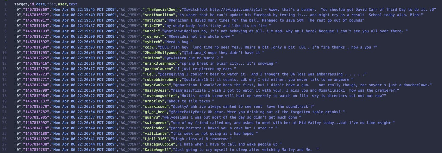
Here is a preview of the dataset:
Step 1: Setup TensorFlow with Metal (optional)
We begin by setting up TensorFlow to leverage the GPU, if available, for improved performance. This setup includes configuring TensorFlow to dynamically manage GPU memory, allowing it to grow as needed. Using the GPU instead of the CPU significantly speeds up model training, especially for large datasets.
import os
import tensorflow as tf

# Set up GPU if available
os.environ['TF_FORCE_GPU_ALLOW_GROWTH'] = 'true'

gpus = tf.config.list_physical_devices('GPU')
if gpus:
    try:
        for gpu in gpus:
            tf.config.experimental.set_memory_growth(gpu, True)
        print("Using GPU:", tf.config.list_physical_devices())
    except RuntimeError as e:
        print(e)
else:
    print("No GPU found. Using CPU instead.")
Step 2: Load the Data
Next, we load our tweet dataset. For the purpose of making this easier to work with, we're only loading in the data that we need from the dataset. In this case, the text and sentiment columns. I’m using Pandas to load the data and manipulate it.
import pandas as pd

data = pd.read_csv('data/tweets.csv')
target_and_text = data[['target', 'text']]

print(target_and_text.head())
Here is an example of what the structure of the data will look like:
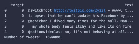
“target” is the sentiment of the tweet. If the value is “0” the sentiment is negative, and if the value is “4” the sentiment is positive. This dataset also claims to have neutral tweets represented by “2”, however, I can’t find any rows in this dataset with a target of “2”. Hmm, weird.
Step 3: Organise the Data
Organising the data before processing it can make the process of building a model so much easier. I started by randomising the order of the rows in the dataset. I've done this to prevent the model from detecting patterns in the order of the data and/or any ordering of the data having an influence on the training of the model. In the case of this dataset, the first 800,000 rows contain negative tweets, and the final 800,000 rows contain positive tweets, so randomising these tweets is essential.
# Randomize the data
target_and_text = target_and_text.sample(frac=1)

# Split data into training and test sets
test_size = len(target_and_text) // 10
test_data = target_and_text[:test_size]
train_data = target_and_text[test_size:]

print("Number of tweets in test data:", len(test_data))
print("Number of tweets in train data:", len(train_data))
The output of each of the print statements are:
Number of tweets in test data: 160000
Number of tweets in train data: 1440000
Step 4: Preprocess the Data
To clean the tweets, we remove URLs, mentions, hashtags, and punctuation. This preprocessing step is crucial because it eliminates noise in the data, allowing the model to focus on the actual content of the tweets. By removing irrelevant information, we help the model learn meaningful patterns, leading to better predictions.
import re
import string

def clean_tweet(tweet):
    tweet = tweet.lower()
    tweet = re.sub(r"http\S+|www\S+|https\S+", "", tweet, flags=re.MULTILINE)
    tweet = re.sub(r"\@\w+|\#", '', tweet)
    tweet = tweet.translate(str.maketrans("", "", string.punctuation))
    return tweet

train_data['text'] = train_data['text'].apply(clean_tweet)
test_data['text'] = test_data['text'].apply(clean_tweet)
Step 5: Tokenize the Data
We use Keras Tokenizer to convert the text into sequences of integers that the model can process. TensorFlow works with tensors, which are multi-dimensional arrays that allow us to represent our data in a format suitable for neural network computations. By converting text into sequences of integers, we are transforming our data into a format that TensorFlow understands.
You may also notice the "max_features" variable which we are passing to the Tokenizer. This is the number of unique words we want to keep in the vocabulary, chosen based on the most frequent words in the dataset. This helps reduce the size of our vocabulary to include only the most relevant words, making training more efficient.
from tensorflow.keras.preprocessing.text import Tokenizer

max_features = 10000

tokenizer = Tokenizer(num_words=max_features)
tokenizer.fit_on_texts(train_data['text'])

number_of_unique_words = len(tokenizer.word_index)
print("Number of unique words:", number_of_unique_words)

tweet_train = tokenizer.texts_to_sequences(train_data['text'])
tweet_test = tokenizer.texts_to_sequences(test_data['text'])

print(tweet_train[0])
print(tweet_train[1])
For this project, the total number of unique words was 417,153. So only keeping track of 10,000 helps to make the model easier to train, and as I said before, ensures that the model only focuses on the most relevant words in the tweets.
Here are two examples of what tweets would look like after going through this process:
[799, 26, 3, 168, ...]
[11, 2164, 1140, 85, 6235, ...]
Step 6: Pad the Sequences
Now that our tweets have been converted into arrays of numbers, we need to add padding to each of them.
Padding is used to ensure that all input sequences are of the same length, which is essential for batch processing in neural networks. Without padding, the model wouldn't be able to handle inputs of varying lengths efficiently, which could lead to errors during training.
You can see at the top of the code snippet, we calculate the maximum length of the tweets in the training data. In reality, I may have been better off extending the maximum length just in case any of the tweets in the test data are longer, but this wouldn't have much of an impact for a model like this.
from tensorflow.keras.preprocessing import sequence

maxlen = max([len(x) for x in tweet_train])
print('Max length:', maxlen)

tweet_train = sequence.pad_sequences(tweet_train, maxlen=maxlen, padding="post")
tweet_test = sequence.pad_sequences(tweet_test, maxlen=maxlen, padding="post")

# Convert sentiment labels from 0/4 to 0/1
train_data['target'] = train_data['target'].apply(lambda x: 0 if x == 0 else 1)
test_data['target'] = test_data['target'].apply(lambda x: 0 if x == 0 else 1)

sentiment_train = train_data['target']
sentiment_test = test_data['target']

print('sentiment shape:', sentiment_train.shape)
Step 7: Build the Model
We build an LSTM-based model for sentiment classification. The model has 8 different layers. Here's a breakdown of each of the layers.
Input: The input layer accepts sequences of tokenized words, each represented by an integer. This layer defines the shape of the input data, which in our case is a sequence of fixed length (maxlen).
Embedding: The embedding layer converts each word token into a dense vector of fixed size (`embed_size`). This helps the model learn word representations and capture semantic meanings.
Dropout: Dropout helps prevent overfitting by randomly setting a fraction of the input units to zero during training.
LTSM: The LSTM (Long Short-Term Memory) layer captures temporal dependencies in the input sequences, making it ideal for understanding context in the text.
GlobalAveragePooling1D: This layer calculates the average output of the LSTM layer across the time dimension, reducing the dimensionality of the data.
Dropout: Another dropout layer to further reduce the risk of overfitting by adding regularization.
Dense (64): A fully connected layer with 64 units and ReLU activation, which learns complex features from the pooled data.
Dense (1): The output layer with a single unit and sigmoid activation, providing a probability of positive sentiment.
I've compiled the model to use the "adam" optimizer, which is helpful for adjusting the learning rate during training to make the model learn faster and more accurately. The “binary_crossentropy” loss function is used because it is ideal for binary classification tasks like sentiment analysis (e.g. positive or negative). The “BinaryAccuracy” metric measures the percentage of correct predictions, helping to evaluate model performance.
from tensorflow.keras.layers import Input, Embedding, LSTM, Dense, Dropout, GlobalAveragePooling1D
from tensorflow.keras.models import Sequential
from tensorflow.keras.regularizers import l2
from tensorflow.keras.metrics import BinaryAccuracy

embed_size = 10

model = Sequential([
    Input(shape=(maxlen,)),
    Embedding(input_dim=max_features, output_dim=embed_size, input_length=maxlen),
    Dropout(0.2),
    LSTM(64, return_sequences=True),
    GlobalAveragePooling1D(),
    Dropout(0.3),
    Dense(64, activation='relu', kernel_regularizer=l2(0.01)),
    Dense(1, activation='sigmoid')
])

model.compile(optimizer="adam", loss='binary_crossentropy', metrics=[BinaryAccuracy(threshold=0.5)])

model.summary()
Step 8: Train the Model
We train the model using early stopping to prevent overfitting. So if during training, the model does not improve within 3 epochs, it will stop training and revert back to the weights that had the best results.
Epochs are essentially the number of times the model will see the entire training dataset during training, the more epochs we run, the more opportunities we give the model to detect patterns in our data. In this case I have set the number of epochs to 20, however, as mentioned before, early stopping could reduce this number.
import matplotlib.pyplot as plt
from tensorflow.keras.callbacks import EarlyStopping

batch_size = 100
epochs = 20

early_stopping = EarlyStopping(monitor='val_loss', patience=3, restore_best_weights=True)

history = model.fit(tweet_train, sentiment_train, batch_size=batch_size, epochs=epochs, validation_split=0.1, callbacks=[early_stopping])

plt.plot(history.history['loss'], label='Training Loss')
plt.plot(history.history['val_loss'], label='Validation Loss')
plt.xlabel('Epochs')
plt.ylabel('Loss')
plt.legend()
plt.show()
Here is the output of the training data on a chart. We can see that the loss for both the training and the validation data improves consistently for the first 7 epochs, and then at epoch 10 the early stopping function has been triggered.
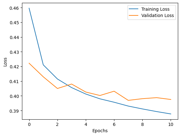
You may be wondering, what does this chart mean? And what is loss?
Loss measures how well the model’s predictions match actual values, while accuracy shows the percentage of correct predictions. During training, we use loss because it provides more detailed information on how wrong predictions are and is differentiable, allowing the optimisation algorithms to adjust the model’s weights effectively. Essentially, loss guides the learning process, while accuracy indicates performance after training.
Step 9: Evaluate the Model
After training, we can evaluate the model on the test data (which the model has never seen before) to measure its performance.
score = model.evaluate(tweet_test, sentiment_test, batch_size=batch_size)

print(f"Test Loss: {score[0]} - Test Accuracy: {score[1]}")
Here is the output of the print statement:
Test Loss: 0.39833131432533264 - Test Accuracy: 0.8204562664031982
This means that the accuracy of the model is 82%. For a lightweight model like this, I’d say that’s a pretty successful result.
Step 10: Manual Testing
Finally, I manually tested the model using some example tweets that I wrote to see how the model performs. I made sure to clean the tweets and process them into padded sequences using the exact same process that I applied to the training data.
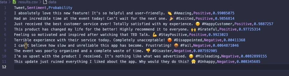
This model doesn't just output a "positive" or "negative" result. It actually outputs a value between 0 and 1 corresponding to how negative (0) or positive (1) the tweet is. So I've added another step which classifies all of the results below 0.5 as negative and all of the results above 0.5 as positive.
I saved the results of this prediction into a CSV file called "data/results.csv".
import numpy as np

# Example tweets for testing
original_tweets = [
    # Positive Sentiment
    "I absolutely love this new feature! It's so helpful and user-friendly. 👏 #Amazing",
    "Had an incredible time at the event today! Can't wait for the next one. 🎉 #Excited",
    "Just received the best customer service ever! Totally satisfied with my experience. 😊 #HappyCustomer",
    "This product has changed my life for the better! Highly recommend it to everyone. 🙌 #Grateful",
    "Feeling so motivated and inspired after watching that TED Talk. 💪 #StayPositive",

    # Negative Sentiment
    "Terrible experience with their service today. Completely unacceptable! 😡 #Disappointed",
    "I can’t believe how slow and unreliable this app has become. Frustrating! 🤬 #Fail",
    "The event was poorly organized and a complete waste of time. 👎 #Disaster",
    "I'm so upset with the product I received. It's nothing like what was advertised. 😒 #Misleading",
    "This update just ruined everything I liked about the app. Why would they do this? 😤 #Unhappy"
]

tweets = [clean_tweet(tweet) for tweet in original_tweets]
tweets = tokenizer.texts_to_sequences(tweets)
tweets = sequence.pad_sequences(tweets, maxlen=maxlen, padding='post')

predictions = model.predict(tweets)

predicted_classes = np.where(predictions > 0.5, 'Positive', 'Negative').flatten()

results = pd.DataFrame({
    'Tweet': original_tweets,
    'Sentiment': predicted_classes,
    'Probability': predictions[:,0]
})

results.to_csv('data/results.csv', index=False)
Here are the outputted results from the manual testing. We can see 3 columns: Tweet, Sentiment and Probability.
It’s interesting to look at the probability stats for each of these tweets.
And there you have it! A complete sentiment analysis model built with TensorFlow that can predict the sentiment of tweets. The code walks through every stage, from loading and cleaning data, building the model, training, evaluating, and finally making manual predictions.
I have published the entire codebase on GitHub. You can find it here: https://github.com/IAmTomShaw/tweet-sentiment-analysis-model
Tom, do you have local GPU or would you run this on a virtual machine in AWS?